


This article gives an example of how profound proximity effects can be.
Introduction
In this article, Dr. Ridley discusses one of the most difficult aspects of magnetics design and analysis: winding proximity loss. Without understanding proximity loss, there is a roadblock to reducing the size of the magnetics components.
The Size of Modern Magnectics
In the last ten years, tremendous strides have been made in semiconductors to increase the performance of high-frequency power supplies. New wide-bandgap technologies, and new packaging techniques have led to unprecedented levels of power density and converter efficiency. The future for power conversion has never been so exciting.
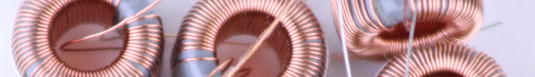
However, one component has stubbornly continued to defy proportional miniaturization—the magnetics. Invented in 1831, the power transformer remains a larger component than anticipated, and it does not seem to follow any version of Moore’s Law.
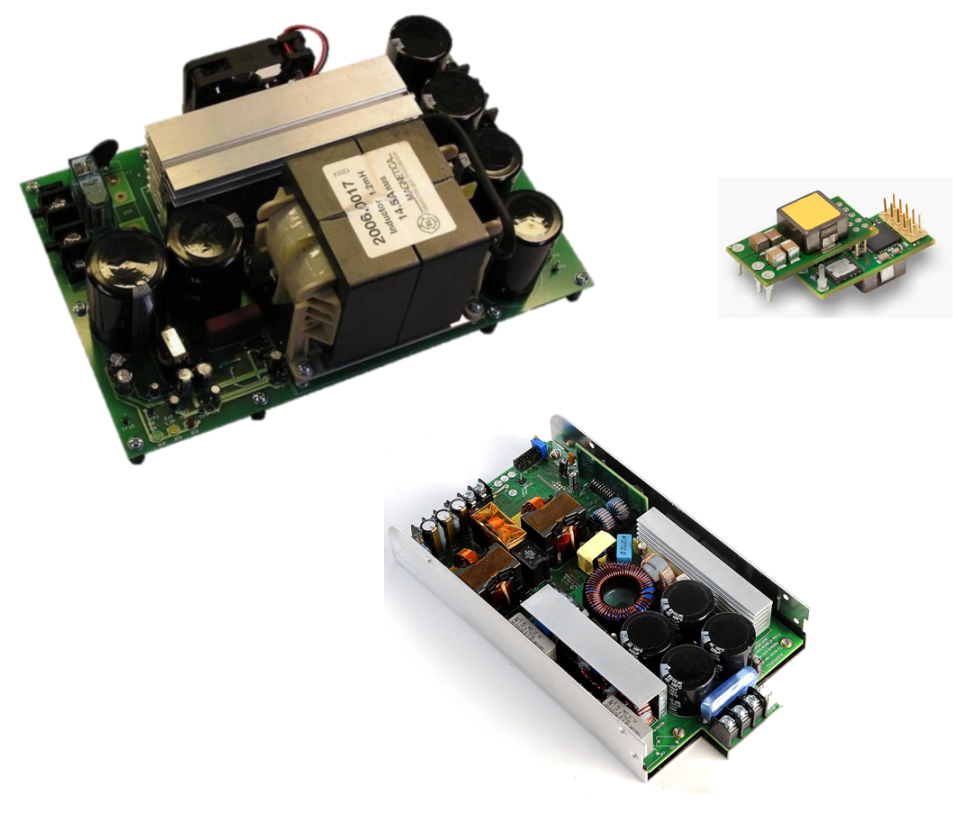
Figure 1: Modern Power Converter Size is Dominated by the Magnetic Components
Figure 1 shows modern power converters for different applications. A PFC circuit, LLC, and a point-of-load converter all feature prominent magnetics. In some cases, we find that the semiconductor devices no longer even need a heatsink and have disappeared from view underneath the circuit board. This emphasizes even more the need to work harder on the magnetics if we are to continue making progress with size reduction.
When starting a series of articles on magnetics design, it is customary to start at the beginning with design basics. Considerations of turns counts, saturation, core materials, and design optimization are usually at the forefront. You can learn more about some of these issues from our magnetics videos [1].
However, in this article, we are going to start with an advanced topic which causes severe problems for many designers. We will see in the example used in this article that conventional analysis of winding loss indicates that there will be just over 1 W of dissipation. However, detailed proximity loss analysis shows that, in reality, there is almost 15 W of power loss.
Forward Converter Design Example
Figure 2 shows an example forward converter running at 360 W. The converter runs at a switching frequency of 100 kHz. We will look at the detailed design of the transformer and show that it demonstrates excessive winding loss, despite initially good performance calculations.
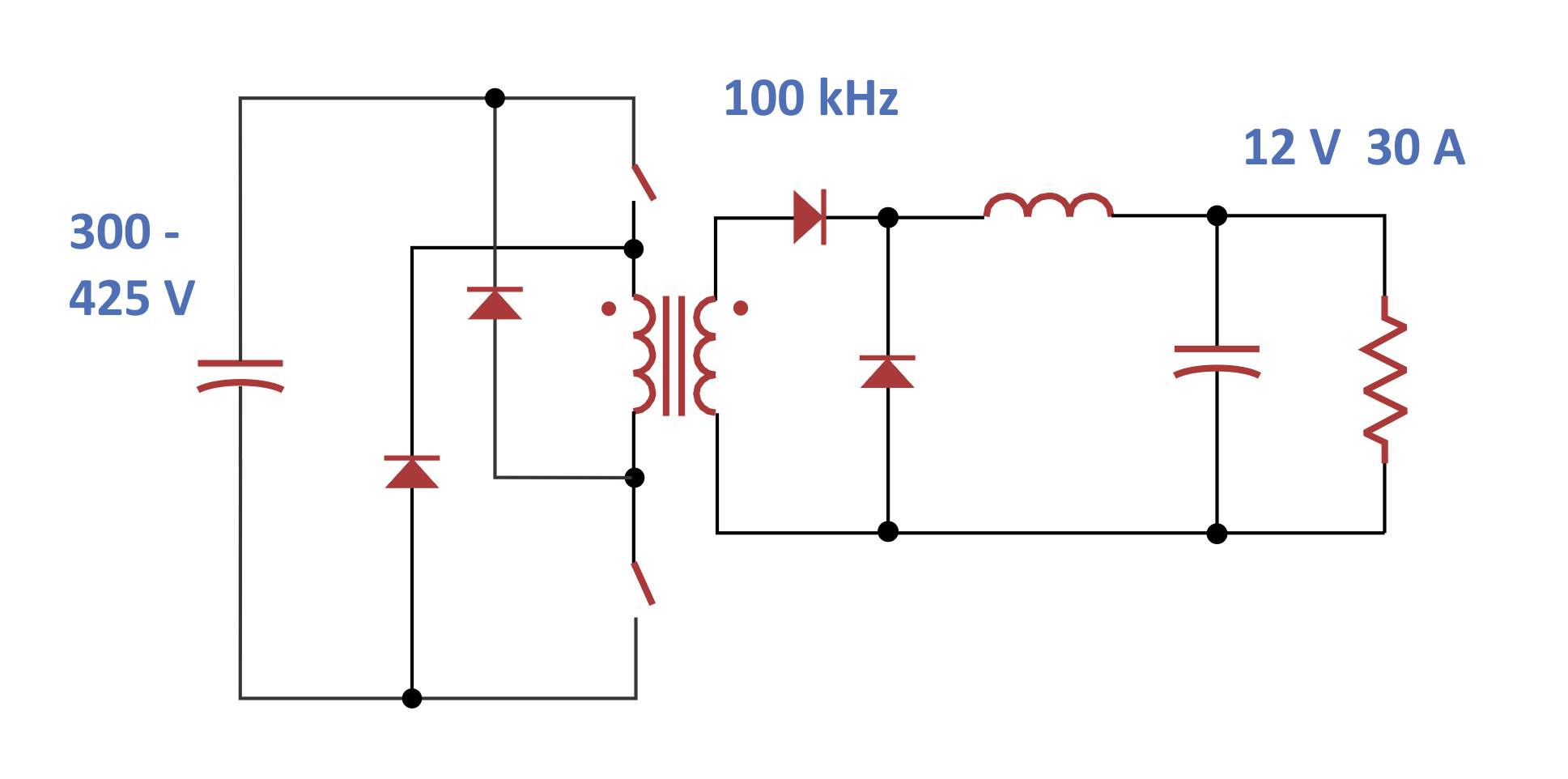
Figure 2: Two-Switch Forward Converter for 360 W Output
Figure 2 shows the simulated currents in the transformer [2]. The primary current has a peak almost 4 A, and an RMS value of 1.985 A. Notice that there is a dc component of the current. (This can be a surprise to power supply novices. Transformers are not ac-current devices, they are ac-voltage devices.) There are also ac frequency components at 100 kHz, 300 kHz, and higher order odd harmonics. As we will see later, different analysis techniques can include these ac components to calculate the total winding loss accurately.
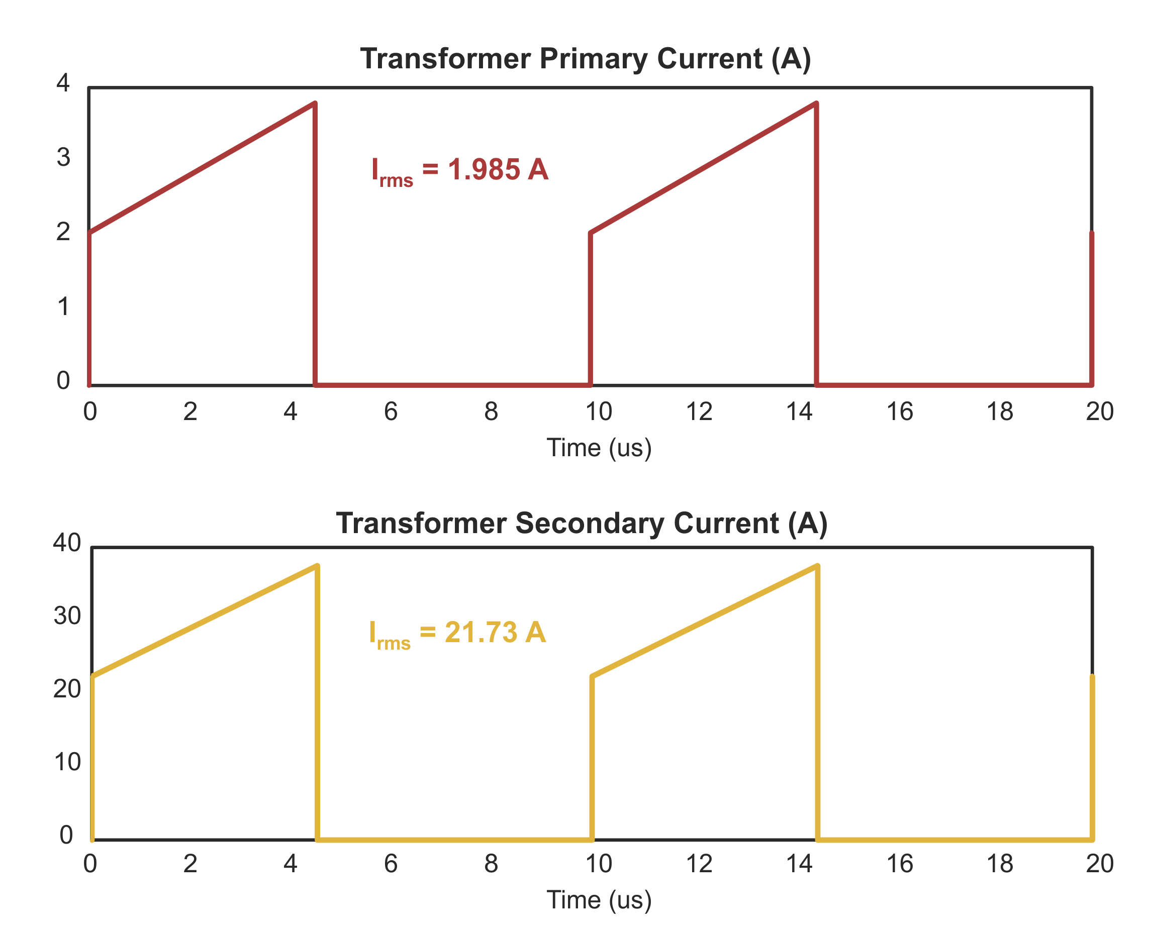
Figure 3: Transformer Currents for the 2-Switch Forward Converter
The secondary waveforms reach a peak of almost 40 A, with an RMS current of 21.73 A. If you look closely at the waveforms, you may notice that the primary slope is slightly higher than the secondary slope. This is due to the addition of magnetizing current in the primary winding. This component is not seen on the secondary side.
Figure 4 shows the detailed winding construction of the transformer in a cross-sectional view.
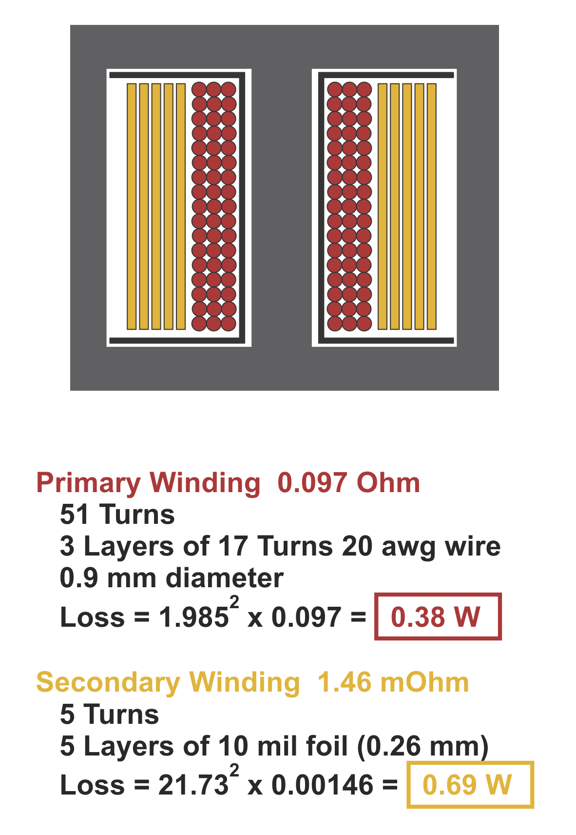
Figure 4: Forward Transformer Design Details and Calculated Winding Dissipations
The primary is composed of 3 layers of 20 awg wire, comprising a total of 51 turns. The total dc resistance is 97 mOhm, and the calculated rms dissipation is 0.38 W.
The secondary is wound with 10 mil foil. This results in 0.146 mOhm dc resistance, with a calculated dissipation of 0.69 W. This total dissipation looks really good, and most engineers will be happy to take this to a prototype design for testing in their project.
AC Resistance Calculations
Most engineers in power are familiar with the fact that the resistance of a conductor changes with frequency. Some advanced math, long established, introduces us to the concept of skin effect where currents at high frequencies move to the surface, or skin, of a conductor. Manufacturers of early high-power distribution transformers were painfully aware of this effect when their transformer windings became hotter than expected.
While most engineers are aware of skin effect, very few of them are familiar with proximity effect. (Skin effect is actually a subset of proximity effect.) With proximity, the currents in a conductor do not flow evenly around the surfaces of a conductor. When wrapped in a helix around a core, the currents will concentrate unevenly on the inner and outer surfaces. With multiple layers of windings, circulating currents are produced. This is similar to induction heating, and the losses can become very large.
The mathematics, involving Dowell’s famous equations, are very complex for calculating ac resistances. The main body of this work was completed in 1961, and is readily available to all engineers. Due to its complexity, less than 1% of power electronics engineers take advantage of this work.
Figure 5 shows the profound results that arise from properly applying Dowell’s equations to the primary windings of the forward converter power transformer. This graph, on a log-log scale, shows the rising resistance of the wire with frequency, plotted from 10 Hz to 10 MHz.
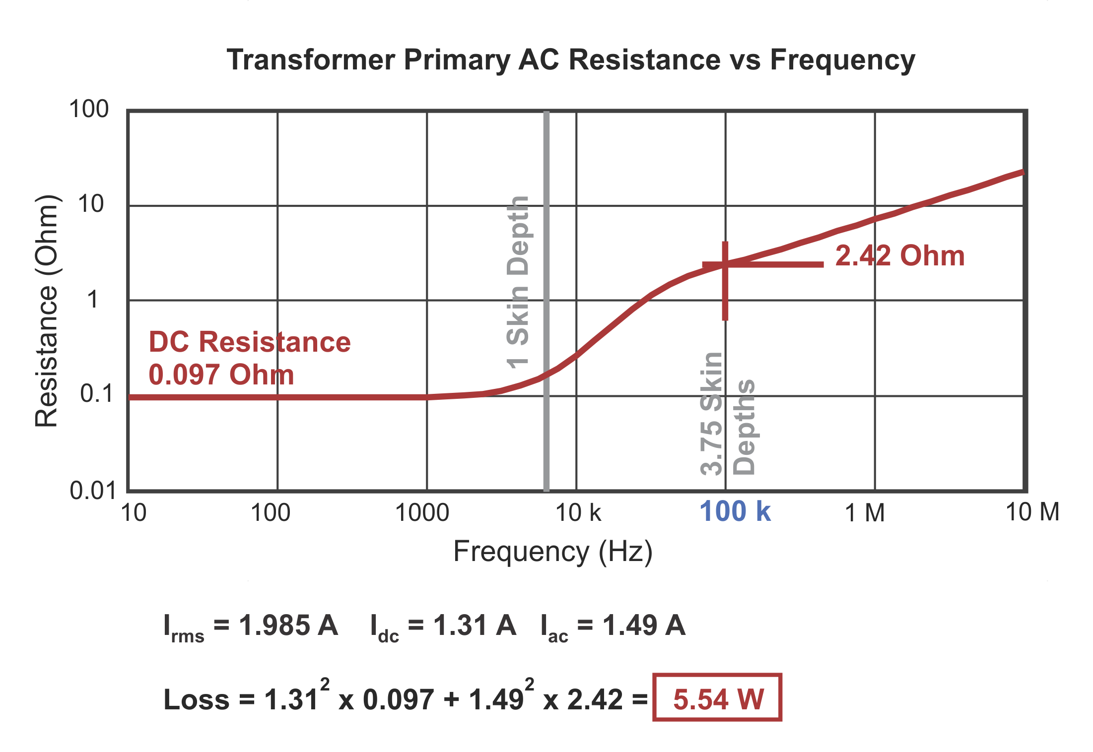
Figure 5: AC Winding Resistance Versus Frequency for the 3-Layer Primary Winding
At low frequencies, the resistance is equal to the calculated dc value, 97 mOhms. At around 7 kHz, the skin depth is equal to the thickness of the primary wire, and we see the resistance start to rise at about 2 kHz. At the switching frequency, 100 kHz, the wire thickness is 3.75 times the skin depth. However, we see that the resistance has risen far more than that. It is now 2.42 ohms, or about 24 times the dc resistance.
We can use this information to approximate the total loss in the wire. This is done by taking the dc component of the current, squared, multiplied by the dc resistance. To this we add the total ac current squared times the ac resistance at 100 kHz. The result is an astonishing 5.5 W of loss, while conventional analysis suggests only 0.38 W.
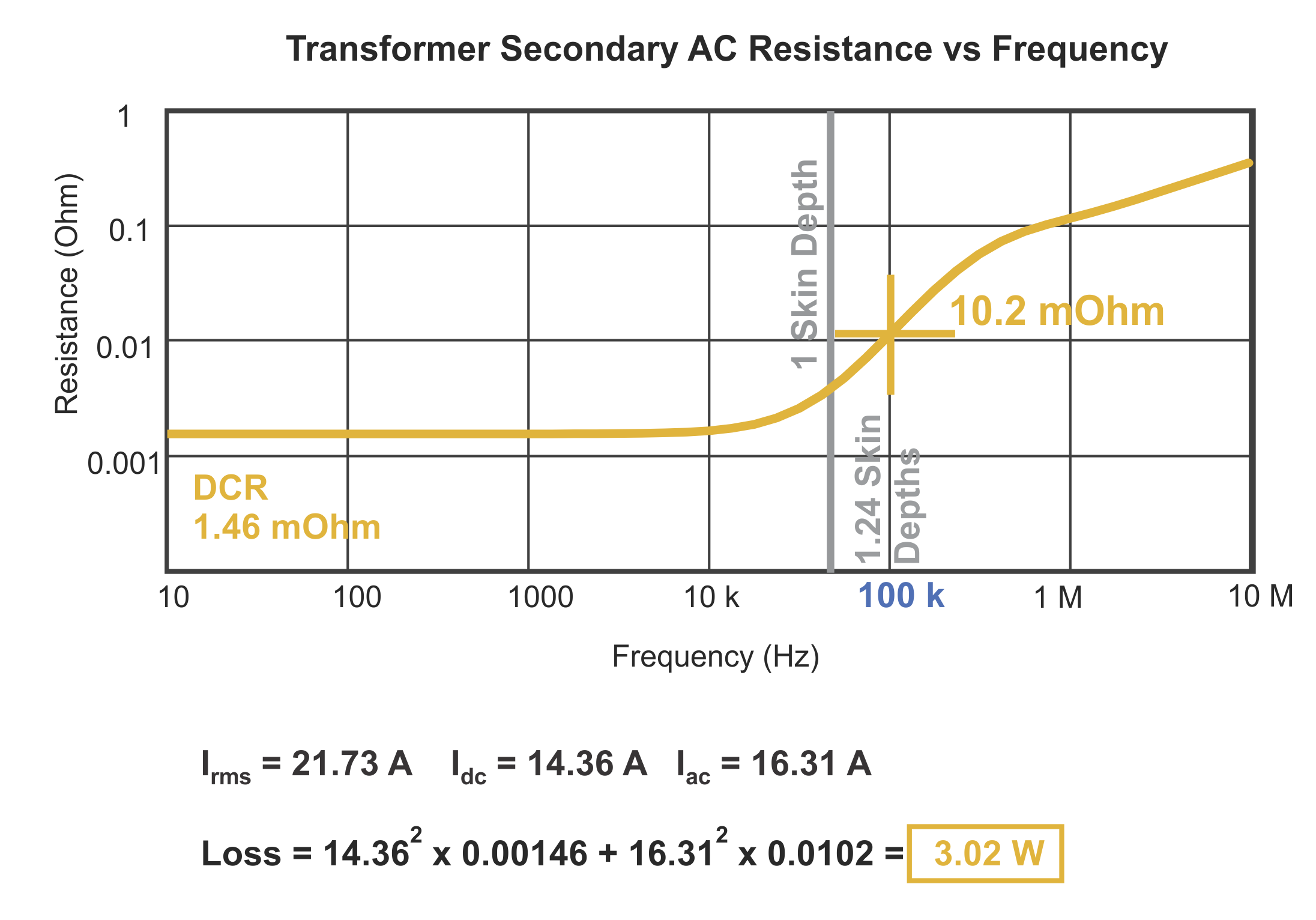
Figure 6: AC Winding Resistance Versus Frequency for the 5-Layer Foil Secondary Winding
We can repeat this process for the secondary winding. Figure 6 shows the ac resistance of the 10 mil foil versus frequency. This is a much thinner winding than the primary, and the skin depth is not reached until we get to about 65 kHz. You can see, however, that the resistance starts to rise well before this frequency, due to the multiple layers of foil. At 100 kHz, the foil is only 1.24 skin depths, but you can see that the ac resistance is about seven times higher than the dc resistance. When we separate the current into ac and dc components, the loss calculates to be about 3 W—almost five times bigger than the calculation without proximity effects included.
Many designers would be misled with this secondary design. An old rule of thumb is that you have to stay below 2 skin depths to avoid problems with your windings. In this case, it doesn’t help. The increased resistance is still a factor of five higher than expected.
Circuit Models Reduce Calculations and Increase Accuracy
Even though the proximity calculations described so far indicate greatly increased losses, they still fall short of the real circuit losses. This is because all of the ac current is assumed to be at the switching frequency. In reality, there are higher harmonics, and the losses will increase further with the increasing resistance.
The difficult and time-consuming way to solve for the winding loss is to extract all of the harmonics from the current waveforms and to calculate the losses due to each frequency component. However, there is a simpler and more powerful way to do this.
The ac resistance versus frequency plots of figures 5 and 6 can be modeled with R-L ladder networks as shown in Figure 7. A sequence of 5 branches is sufficient to follow the curve accurately from 10 Hz to 10 MHz. These linear circuit models can then be simulated in LTspice, or any other circuit analysis package.
The inspiration for the R-L ladder network is drawn from Dr. Vatché Vorpérian’s paper on frequency-dependent core loss [3]. In this landmark paper, he showed how simple circuit models could be used to simulate very complex loss equations, and the same can be done for proximity losses.
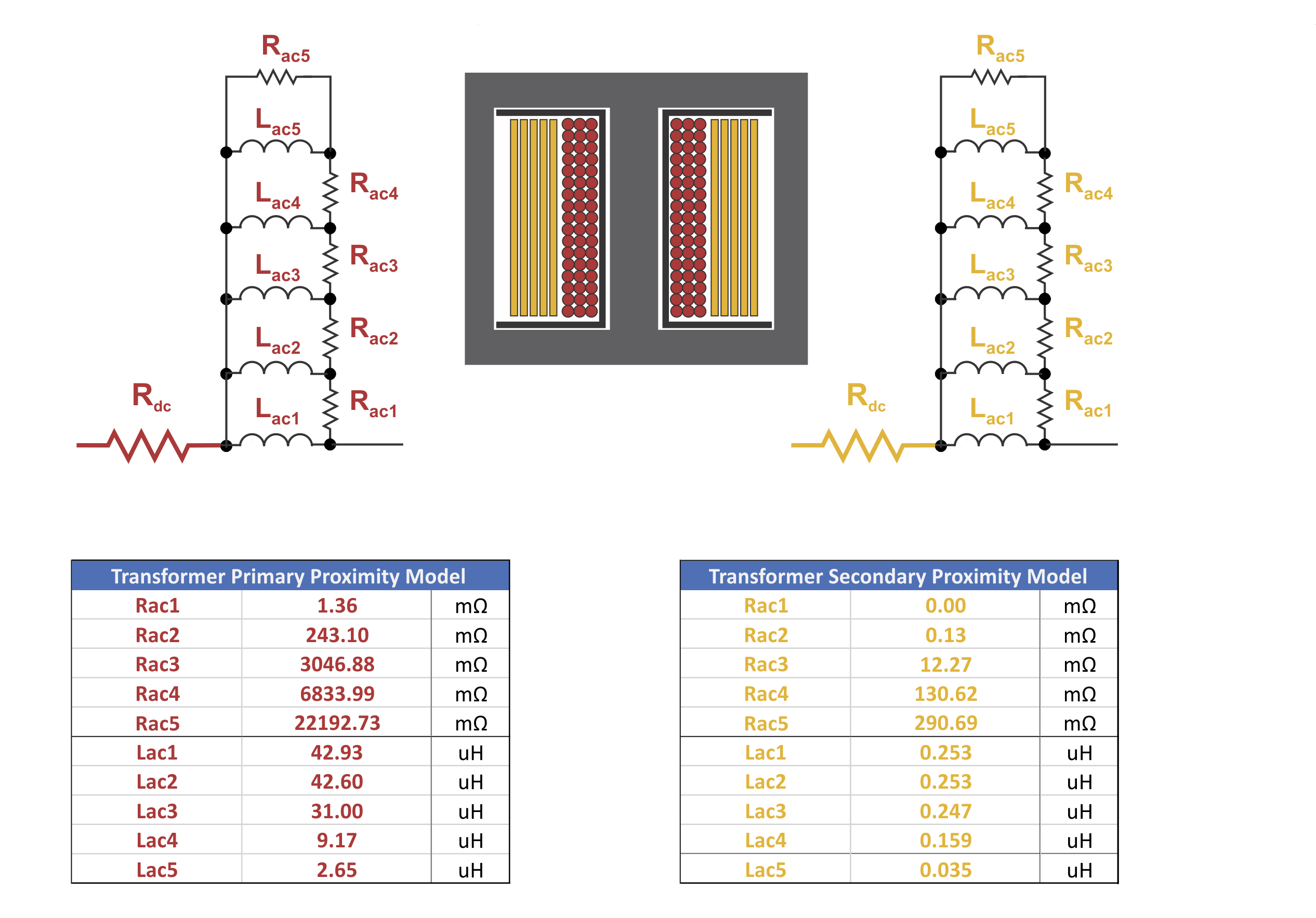
Figure 7: Linear Circuit Networks Are Sufficient to Properly Simulate Proximity Losses
The circuit simulation will automatically steer the transformer current through higher resistances at high frequencies, and no calculation of harmonic content is needed. This happens automatically in the time-domain simulation.
Despite the apparent complexity of the winding equivalent circuits, LTspice does not have any trouble in simulating at a reasonable speed. The results are very revealing. As can be seen from Figure 8, the primary winding loss climbs to 8.46 W, and the secondary to 6.27 W. The resulting 14.7 W is far from the initial loss estimate of about 1 W.
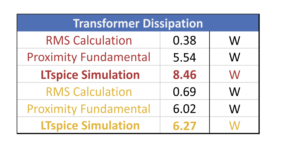
Figure 8: Calculated Winding Losses Using RMS Calculation, Proximity with Fundamental Frequency Only, and LTspice Simulation with Full-Frequency Proximity.
Many designers run into this difficulty with their transformer designs. The excess loss greatly lowers efficiency, and the power supply may not meet its specifications. Furthermore, the 14.7 W loss will raise the temperature of the windings significantly, resulting in still higher winding resistance and loss.
Summary
Dowell’s equations are essential to arrive at the real dissipation in transformer windings. If these calculations are not done, the magnetics winding loss can be an order of magnitude higher than expected. Most engineers do not make these calculations, however, due to the difficulty in understanding the process. Fortunately, modern software [2] is available to automate the entire process of model generation ready for circuit simulation. All that is needed is a description of the winding structure to generate accurate LTspice models. It is then easier, with any level of experience, to accurately predict dissipation and temperature rise in a transformer.
Even more importantly, a transformer can be redesigned with less layers to improve the dissipation in the windings. This will be illustrated in a future article.
References
-
Magnetics Design Videos, Ridley Engineering Design Center.
-
Power 4-5-6 Simulation software.
-
Dr. Vatché Vorpérian, “Using Fractals to Model Eddy Current Losses in Feretic Materials,” Switching Power Magazine 2006.
-
Learn about proximity losses and magnetics design in our hands-on workshops for power supply design www.ridleyengineering.com/workshops.html
-
Join our LinkedIn group titled Power Supply Design Center. Noncommercial site with over 7100 helpful members with lots of theoretical and practical experience.