


Calculating the difference between sinewave and triangle wave excitation shows that sinewave measurements are sufficient for loss calculations.
Introduction
The first two parts of this article showed how the core losses for real waveforms could be modeled better. In the first part, a continuous expression was used to model a wide range of excitations. In the second part, the effect of duty cycle on the loss of the core material was included in a single equation. In this third and final part, we return to the discussion of the sinewave versus the triangle wave excitation to analyze the difference between the two for a given material.
Adaptive Steinmetz Equation
Part I of this article [6] showed how a single adaptive equation could be used for predicting the core losses of a ferrite material. Figure 1 shows the specific equation for the Magnetics “R” material. The equation adapts itself to the changing slope of the curves with frequency, providing a continuous equation for all frequencies.
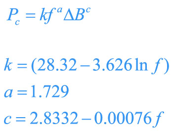
Equation 1: Core Loss Equation for R Material and All Frequencies
Having a single equation is very important for extending core-loss analysis into duty-cycle effects, and for making the incorporation of core loss into design programs manageable.
Sinusoidal Core Excitation
All core loss curves are measured using sinusoidal excitation. However, in squarewave converters, the excitation of the core is not sinusoidal at all. A 50% square wave voltage drive results in a triangular current waveform in the inductor, and a triangular waveform for the core excitation. Figure 1 compares a sinusoidal excitation with a triangle wave excitation. Notice that both waveforms of Figure 2 have the same peak value, or the same peak flux excitation.
As mentioned in part II of this series, Mr. Rudy Severns demonstrated many years ago that the difference in loss is small between a sinusoidal excitation and a 50% triangle wave. The waveforms of Figure 1 give an indication of why this happens. For part of the waveform, the sinusoidal curve has a lesser slope than the triangular, and for other parts, the slope is greater.
In this article, we will go ahead and confirm numerically the difference for the Magnetics R material.
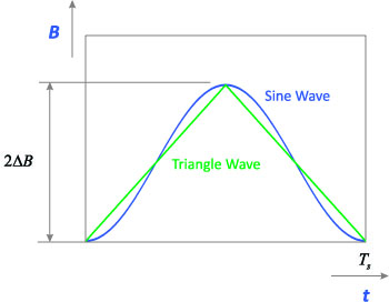
Figure 1: Sinusoidal and 50% Duty Cycle Triangular Waveforms
Calculating Sine and Triangle Waveform Difference
To calculate the actual loss of the two different waveforms, we can use the apparent frequency approach discussed the Part II of this core-loss series. Instead of using a duty cycle of the waveforms, we can look at the slopes of the sinewave versus the triangle wave, as shown in Figure 2, to modify the calculation frequency.
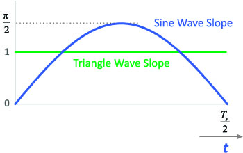
Figure 2: Slopes of the Sine and Triangle Waveforms with Same Peak Flux Excitation.
We have to something a little unusual to proceed. We will assume that the triangle excitation is the base case for which data is collected to show how the varying slope of the sine wave affects the dissipation. (In reality, it is a sinewave.) While this is not a rigorous approach mathematically, it is a good way to demonstrate the differences in the two waveform dissipations in light of the very nonlinear equations involved.
“Apparent Frequency” Loss Calculations for Sinusoidal Waveforms
It was discussed by Cliff Jamerson [2] that the increased loss with fast rise and fall times can be addressed with the method of apparent frequencies. If we look at the slope of the sine wave relative to the triangle wave, shown in Figure 2, we can actually calculate the differences in loss. In the last part of this series, we showed the loss with different duty cycles could be found by inserting different frequencies into the loss equation, resulting in Equation 2.
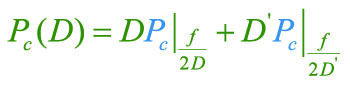
Equation 2: Loss Equation for Different Duty Cycles and Different Apparent Frequencies
We can use a modified form of this equation to calculate what will happen over a half-cycle of the sine wave. Since the equations are nonlinear we cannot use integration to find the results. Instead, we can break the problem into a sequence of summations to approximate the answer. Instead of working with duty cycles, we use the slope of the sinusoidal waveform relative to the triangle wave, and this results in Equation 3 for the first 90 degrees of the waveform
. 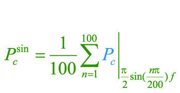
Equation 3: Calculating the Loss of a Sinewave by Breaking the First 90 Degrees in 100 Pieces
Equation 3 was entered into an Excel spreadsheet for calculation. The results are shown graphically in Figure 3. The percentage increase in loss with a sinewave changes with frequency, but does not exceed 14% for the particular example shown. This number can now be used to calculate the actual core loss from the manufacturer’s data. All we have to do for a triangle wave is take the data from the manufacturer’s core loss curves, and divide by the number from the curve of Figure 3.
Please note that this is not a general result that can be used for every material or every excitation level. It is specific to the R material, with an excitation of 0.2 T (that is, a peak-to-peak of 0.4 T). All materials will have their own unique curves for the incremental loss.
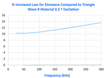
Figure 3: Increased Loss of the Sinewave versus the Triangle Wave with the Same Peak Flux Excitation
Summary
In this sequence of three articles, several things have been shown:
The Steinmetz equation, commonly used to represent core loss, can be expressed as a single equation for all frequencies by having continuously variable coefficients. (Most manufacturers have discrete ranges for different frequencies which produce discrete jumps in predictions and are inconvenient to apply.)
The concept of apparent frequency can be applied to show the increased prediction of loss from the modified and adaptive Steinmetz equation for flux waveforms that are asymmetrical.
The apparent frequency concept can also be applied to show the difference in loss between the 50% triangle waveform and the sinusoidal waveform. This difference is relatively small. Applying the manufacturer’s core material data will result in an overestimation of the actual loss.
All of these effects have been known for some time, but core manufacturers have been slow in applying them to give designers more useful information. A useful step for the industry would be for manufacturers to supply all core loss data (not just curves) and improved modeling in the data books. This would be an ideal project for a graduate student working with one of the ferrite manufacturers.
Another topic which has not been broached here is the effect of temperature on core loss. Many users of power ferrites use the material at extended temperature ranges and do not have the data that they need to calculate losses properly. Designers are also very concerned about efficiency and a full set of data at different temperatures is needed. It is not enough to just provide the data at a couple of temperature points. This topic has been discussed in our Design Center [7].
References
Simulation and Design Software POWER 4-5-6 incorporating Ridley-Nace core-loss equation http://www.ridleyengineering.com/software/POWER_4-5-6_Manual.pdf
Targeting Switcher Magnetics Core Loss Calculations, Clifford Jamerson, Consultant, Power Electronics Technology, Jan 2001.
Join our LinkedIn group titled “Power Supply Design Center”. Noncommercial site with over 7000 helpful members with lots of theoretical and practical experience.
See our videos on power supply design at http://www.youtube.com/channel/UC4fShOOg9sg_SIaLAeVq19Q
Power supply design workshops including magnetics design http://www.ridleyengineering.com/workshops.html
Adaptive Modeling Equation for Core Losses, http://www.ridleyengineering.com/design-center.html Article [89] Core Loss Modelling and [90] Core Loss Modeling Part II Non-Sinusoidal Waveforms
Temperature effects on core loss modelling [A03] Modeling Ferrite Core Losses