


Why Nyquist diagrams are not a very practical measurement.
Introduction
This article shows the link between loop gain Bode plots and Nyquist diagrams. The Nyquist diagram is a subset of the Bode Plot, omitting crucial design data. The linear scaling of the Nyquist diagram restricts its practicality, and omission of frequency as an explicit variable in the plot is a major drawback.
Loop Gain Measurements in Modern Control Systems
In control courses in universities around the world, Nyquist plots are used as a tool to assess stability. They work well with prescribed and well behaved finite-gain analytic transfer functions and many theoretical and interesting homework problems can be created.
However, for working engineers, hardware frequently does not behave as expected. Analytical models are often inaccurate, and pole-zero locations or transfer functions of the power stages are often unknown. In such situations, it is a challenge to predict stability and optimize a closed-loop system. This is where the Bode plot of the loop gain is tremendously useful [1].
But what about Nyquist diagrams in the real world? I have never actually been in a lab where someone wanted to present measurement data as a Nyquist diagram, and there are solid reasons for why this is so. These are:
- Nyquist diagrams are concerned with -1 point encirclements, and hence the low gain region of the plot must be clearly shown. To do this, only the region from a gain a little bigger than 1 is shown. Since the plots are always on a linear scale this greatly restricts the available data shown.
- Nyquist diagrams plot real and imaginary parts of the gain, with frequency as a running parameter. Hence the frequency information is completely missing from the Nyquist plot.
- Two very different systems with completely different crossover frequencies can have identical Nyquist diagrams. This is no help when trying to improve system performance.
- When RHP zeros are present in a system (very common for power supplies) the rules for Nyquist become complex.
- If delays are present in a system the Nyquist criteria are again complicated.
- Integrators, or even double integrators (seen in PFC circuits), provide another level of complication in completing the Nyquist contour.
The complexities of rules that go with the Nyquist diagram are difficult to unravel. Study of many online tutorials about the topic are hard to find when dealing with RHP zeros and integrators. Since these comprise the majority of switching power supplies with feedback, application of Nyquist in the lab is very rare.
Loop Gain Measurement Point
Figure 1 shows a buck converter controlled with a current-mode loop and an outer voltage feedback loop. This is a very common control setup for modern power supplies. The feedback compensation can be implemented in a digital controller, or with analog components as shown.
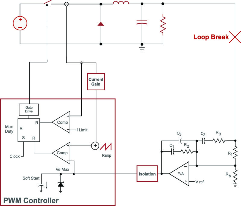
Figure 1: Power supply with current-mode control, showing loop measurement point. .
To assess the stability of this system, it is common in industry to break the loop at the point marked with the red “X”. This can be done with a frequency response analyzer as described in [2].
Bode Plots and Nyquist Diagram Examples for Current-Mode
The design software POWER 4-5-6 [3] has always provided the loop gain Bode plot, and recently a Nyquist diagram has been included for those engineers that wish to see the correlation between the two approaches. All of the plots in this article are generated by the software.
Figure 2 shows a typical loop gain for a current-mode system. The loop sweep starts at 10 Hz so that we can see gains at line frequencies, and continues out to twice the switching frequency.
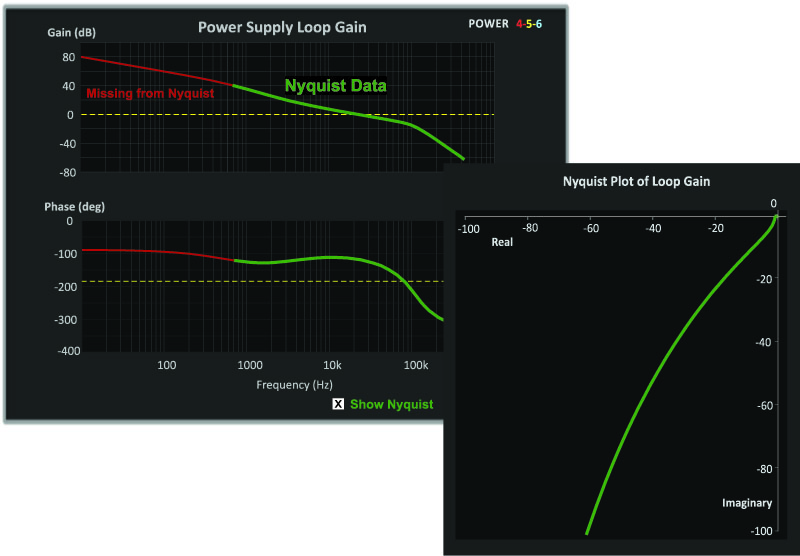
Figure 2: Loop Gain Measurement and Nyquist Plot Generated by POWER 4-5-6. Unit Circle Cannot be Seen on This Scale.
Since the Nyquist plot is done on a linear scale, we have to choose the axis scaling to include a reasonable portion of the Bode plot. If the maximum real and imaginary axes are set at 100, this corresponds to a gain of just over 40 dB. The resulting Nyquist plot is given in Figure 2. Notice that a large part of the Bode plot data, shown in red, is missing from the Nyquist plot. With the linear scale set to these values, the -1 point is compressed into just 1% of the horizontal axis, so this plot is not particularly useful for stability assessment.
With many power systems, if the analog feedback incorporates noise, or the digital feedback is not implemented properly, the gain can flatten out somewhere around a maximum of 40 dB, compromising the performance of the supply. It is important to verify that the gain is higher than this at low frequencies, to make sure the controller is operating properly.
Figure 3 shows the Bode and Nyquist plots of the loop gain with the scale of the Nyquist expanded further. Now only loop data from 20 dB gain and lower is included, but we can begin to see the -1 point more clearly on the Nyquist plot.
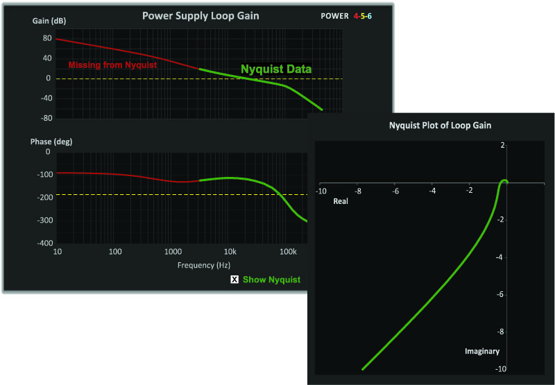
Figure 3: Bode Plot, and Nyquist Plot With Axis Set to Maximum of 10. Maximum Gain is Now Just Above 20 dB.
Figure 4 shows a more common selection for the Nyquist axis scaling. The maximum gain shown is now 10 dB. The advantage of this third plot is that the unit circle and events around the -1 point are now clearly shown. The penalty is that almost all of the data above 0 dB is excluded from the plot, even though this data is very important in optimizing a loop gain. The Nyquist plot is providing only stability data, and little else.
When the green curve of the Nyquist plot crosses the unit circle, the phase of the system above -180 degrees (angle of vector with the negative real axis) can be measured. Of course, this information is directly available from the Bode plot, including the frequency at which the 0 dB crossing occurs.
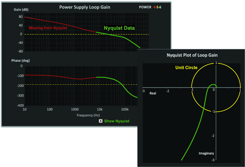
Figure 4: Bode and Nyquist Plot Zoomed In to Maximum of 3 (10 dB). Unit circle is now apparent, and this is the usual kind of scale chosen for Nyquist plots of the Loop Gain.
Summary
In this article, it has been shown how the Nyquist plot is just a subset of the full loop gain data. The data is shown in its entirety by the Bode plot. The Nyquist diagram suffers from two major problems: using a linear scale for the axes, and completely eliminating the frequency information from the plot. There are a few interesting cases where the Nyquist diagram can apply clear rules for stability that are less complex that the Bode plot rules for those cases, but in general for power supplies, the Bode plot is far more useful.
If you would like to discuss topic like these with Dr. Ridley and other industry experts, please join the Power Supply Design Center LinkedIn Group [4].
References
- Join our LinkedIn group titled “Power Supply Design Center”. Noncommercial site with over 7000 helpful members with lots of theoretical and practical experience.
- For power supply hands-on training, please sign up for our workshops.
- “Interpreting Loop Gain Measurements”, Article [77]