[114] Transient Loop Sweeps Outperform Small-Signal Models

Part II: Swept loops in LTspice® provide more accurate and useful results than small-signal models.

Authors: Dr. Ray Ridley, Art Nace and John Beecroft

Ridley Engineering, Inc. Camarillo, California USA

Introduction

In our last article, we showed how LTspice® could be used to simulate clean and dependable Bode plots for switching power supply designs. The technique of combining knowledge of the operation of real-world analyzers with the built-in features of LTspice® allowed us to do this faster and more reliably than ever before.

In this article, we show how swept loops surpass the performance of small-signal analysis. For the first time, we can answer important design questions for high-performance power supplies.

Buck Converter Test Circuit

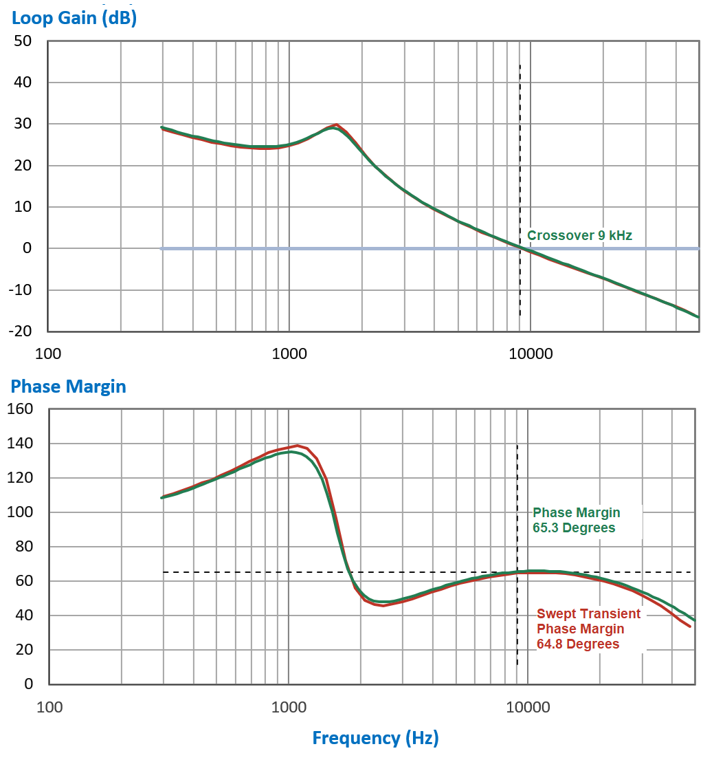
The result of the small-signal model sweep is shown in Figure3. The crossover frequency was 9 kHz with a phase margin of 65.3 degrees, indicating a rugged loop design. (The simulation time was less than one second, demonstrating one of the powerful benefits of using small-signal models.)

The red curve in Figure 3 is the result of sweeping the circuit of Figure 1 without generating small-signal models. You can see that there is almost perfect agreement between the two curves, with only a 0.5-degree discrepancy at the crossover frequency. When approaching 50 kHz ( half the switching frequency) there is a somewhat larger discrepancy in the phase response.

The simulation and processing time for the swept transient circuit was 5 minutes 20 seconds. Analyzer settings were used to obtain the smoothest curves possible rather than the shortest simulation time.

At this crossover frequency design point, either the fast small-signal circuit, or the swept transient circuit provide proper results for assessing the design.

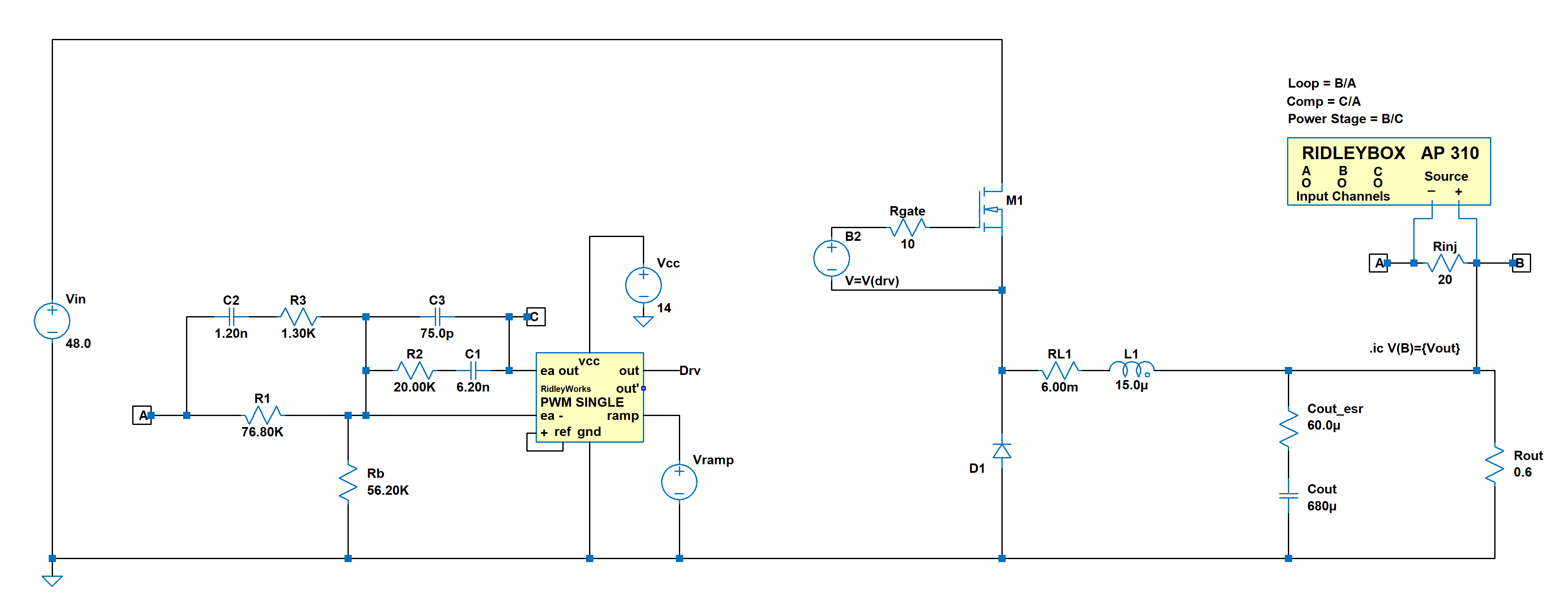
The buck converter is the most prolific topology in power these days since they are being used in huge quantities for point-of-load applications. The test circuit we will consider is a buck converter operating at 100 kHz. The load is 12 V, 20 A, and the input voltage is a nominal 48 V. Figure 1 shows the complete circuit, including feedback components for a loop crossover of 9 kHz. It is the industry norm to put the crossover frequency at 1/10 of the switching frequency but there is a great deal of interest these days in raising it higher. A higher crossover results in smaller output capacitance for a transient load. In this article, we will try to answer an important question: How high the crossover frequency can be raised before encountering instability?

Figure 1 shows the transient simulation circuit for the buck converter, with the model of the RidleyBox®/AP 310 conFigured to measure the loop gain. This process was explained in reference [2].

Figure 1: Buck converter test circuit with Frequency Response Analyzer subcircuit in LTspice®

Small-Signal Circuit with Vorpérian Switch Model

The conventional approach to analyzing the control loops of converters was put in place by Vorpérian in 1986 with his seminal work on the PWM switch model [3]. After the addition of a current-mode extension in 1989, almost nothing has changed since then. We now have many years of multiple dissertations and books covering the same ground, applying the model to different situations.

While the small-signal models are enormously useful, they do suffer from fundamental limitations that are rarely talked about or explored. The mathematics required to fill the gaps are complex, and too particular to any given converter situation. We will explore those limitations here.

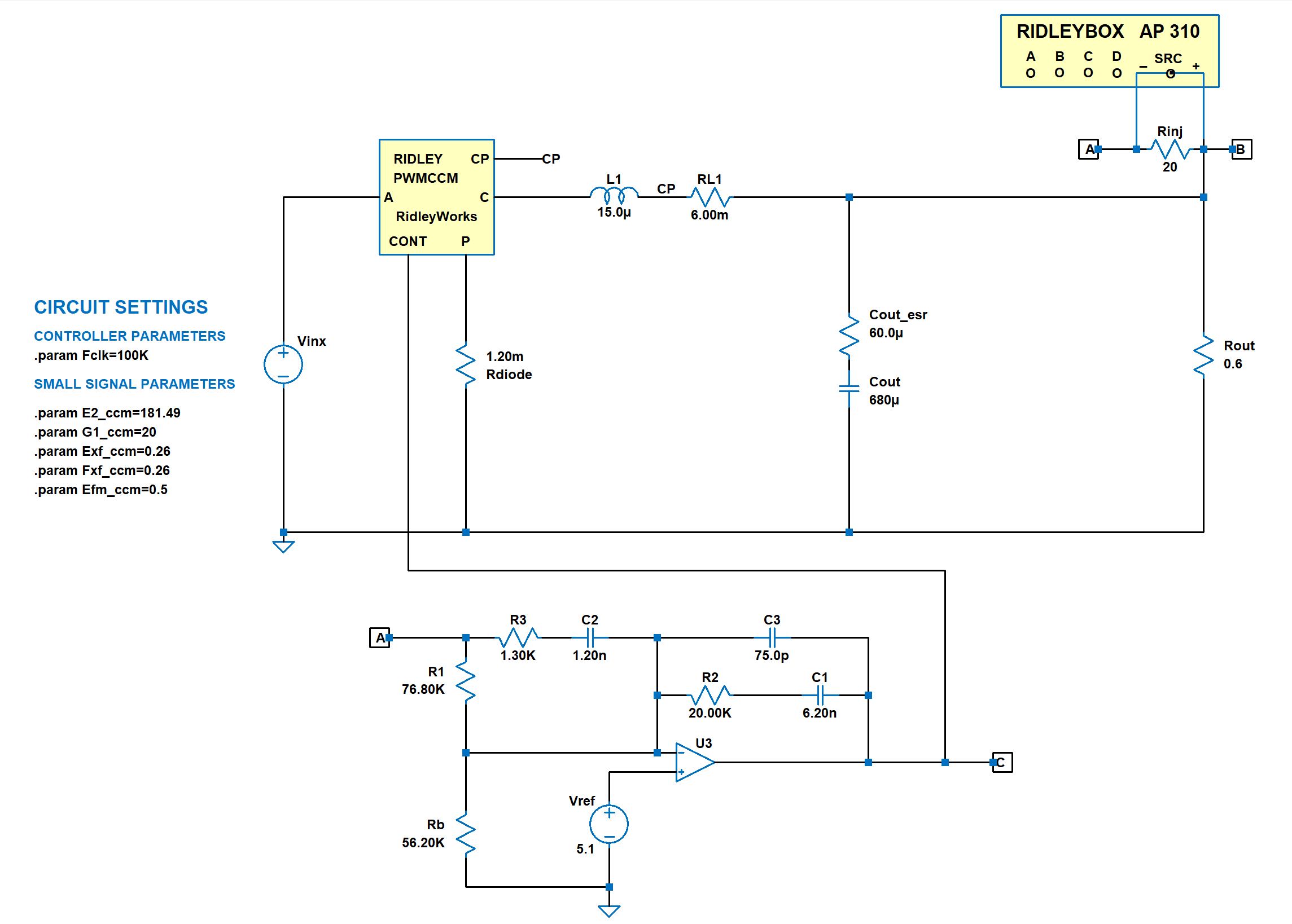
Figure 2 shows the Vorpérian switch model with the parameters of the converter in Figure 1. LTspice® rapidly solves the ac analysis of this circuit, producing the needed plots from the analyzer subcircuit shown.

The internal circuit parameter values are shown under the circuit settings heading on the schematic. These define the small-signal operating point of the circuit for the given load and input line. This entire model schematic is generated automatically by the software program RidleyWorks® [4].

Figure 2: Small-signal model of the buck converter of Figure 1

The result of the small-signal model sweep is shown in Figure3. The crossover frequency was 9 kHz with a phase margin of 65.3 degrees, indicating a rugged loop design. (The simulation time was less than one second, demonstrating one of the powerful benefits of using small-signal models.)

The red curve in Figure 3 is the result of sweeping the circuit of Figure 1 without generating small-signal models. You can see that there is almost perfect agreement between the two curves, with only a 0.5-degree discrepancy at the crossover frequency. When approaching 50 kHz ( half the switching frequency) there is a somewhat larger discrepancy in the phase response.

The simulation and processing time for the swept transient circuit was 5 minutes 20 seconds. Analyzer settings were used to obtain the smoothest curves possible rather than the shortest simulation time.

At this crossover frequency design point, either the fast small-signal circuit, or the swept transient circuit provide proper results for assessing the design.

Figure 3: Loop plots from the small-signal model and the swept transient circuit.

Increasing the Loop Gain of the Small-Signal Circuit

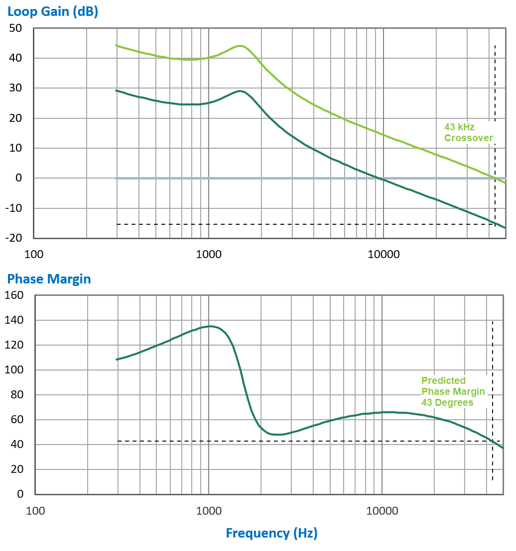
The gain of the feedback compensator can be changed to push the crossover frequency to 43 kHz. As you can see from Figure 4, the phase curve remains invariant. this indicates that there will be a 43-degree phase margin at this crossover frequency. Most small-signal modeling papers for power converters will state that the models are only good for low frequencies, but they are not specific about exactly what that implies. Errors are expected at higher frequencies.

The small-signal loop gain would also indicate that there would be substantial phase margin at 50 kHz. We know from Nyquist that this cannot be true – the phase margin will always be zero at half the switching frequency.

Figure 4: Small-signal model prediction for 43 kHz loop crossover

Increasing the Loop Gain of the Swept Transient Circuit

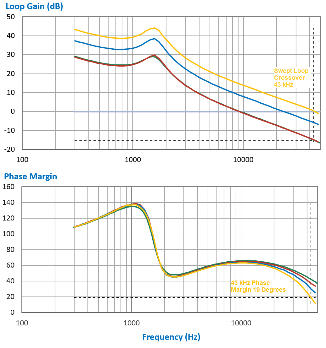
For the swept transient circuit, we obtain much better phase information. There are three swept transient curves shown in Figure 5: the red curve crosses over 0 dB at 10 kHz, the blue curve at 25 kHz, and the gold curve at 43 kHz. The green curve shows the data from the small-signal model. Each of these curves has a different prediction of what the phase margin of the system would be at 43 kHz.

As the crossover frequency of the swept transient curves increases, the phase of the loop deteriorates substantially at higher frequencies. At the 43 kHz crossover frequency (gold curve), the phase margin of the loop is only 19.5 degrees - an unacceptably low value.

Note that great care must be taken when sweeping systems that are close to instability. In this case, the signal injection size was started at 600 mV, and reduced to just 3 mV at higher frequencies. More details of the variable source are given in [2].

Figure 5: Swept loop gain and phase with increasing crossover frequencies

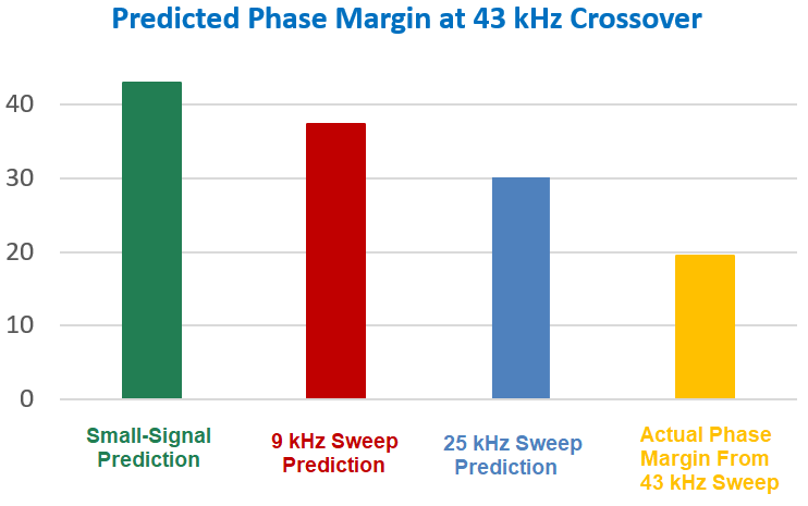
Figure 6 shows clearly shows the error in loop prediction for the small-signal model. There is more than 25 degrees of error versus the actual 43 kHz transient loop sweep.

Figure 6: Phase margin predictions at 43 kHz crossover. The small-signal model gives 25 degrees of error.

Now we have the interesting situation that the original transient circuit is giving much better results than the small-signal model. This is even more intriguing when you realize that it requires no analytical effort to generate the circuit to be swept. What is typically regarded as a “brute-force” approach to design curves is fundamentally superior to the much-researched analytical solutions. Good news for working engineers!

You can also estimate from the curves of Figure 5 that it would be possible to increase the crossover frequency to just above 30 kHz while maintaining a 45-degree phase margin. This is useful design information that is not available from the analytical methods of small-signal modeling.

Figure 6 shows clearly shows the error in loop prediction for the small-signal model. There is more than 25 degrees of error versus the actual 43 kHz transient loop sweep.

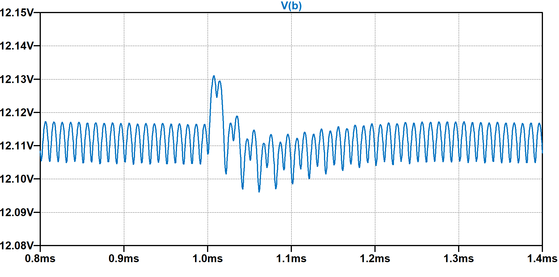
Figure 7: Step-load response clearly showing oscillatory behavior.

Summary

The method of sweeping transient simulation circuits to obtain loop gains is a rugged way to look at the stability of your power converter without having to generate sophisticated small-signal models. It is also more accurate than the small-signal modeling approach, especially as the performance of a loop is pushed to its limits.

The swept transient loop gains clearly show the phase deterioration of the loop as the gain of the circuit is increased. This is a powerful feature, allowing you to accurately predict the stability of your system at higher performance levels.

References

[1] Building a Frequency Response Analyzer in LTspice® by Mike Engelhardt

[2] RidleyBox and AP310 Emulators in LTspice® Design Center Article

[3] Vorperian Switch Model Review Power Supply Design Center Article 69

[4] Design and simulation using RidleyWorks®

[5] Hands-On Power Supply Design Workshops

[6] Join our LinkedIn group titled Power Supply Design Center. Noncommercial site with over 10,000 experienced and helpful industry experts.

[7] Join our Facebook group titled Power Supply Design Center. Advanced in-depth discussion group for all topics related to power supply design with over 5,000 industry experts .