


The standardized curves of Dowell’s equations are a superb tool for designing better high-frequency magnetics. A careful balance of layer count and wire or foil count is needed to reach an optimum design.
Dowell’s Equations
In 1966, Dowell published his famous paper about high frequency losses in multilayer magnetics windings. Despite this happening so long ago, very few engineers working in power electronics today use them in their work. From surveying our thousands of workshop [3] attendees over the years, we estimate the number of engineers using Dowell’s equations to be about 1% of working engineers.
Why is this number so low? When you look at the form of the equation in Figure 2, you get a good idea. The functions in the equation are neither familiar nor intuitive. It takes a lot studying and dedication to learn exactly how to apply the equation to a given situation to find out what losses are going to be.
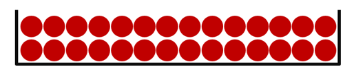
Figure 1: Cross-section of a two-layer winding in a bobbin
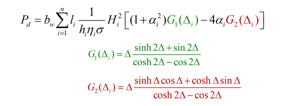
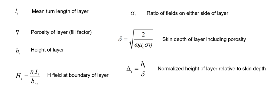
Figure 2: Dowell’s Equation Published in 1966
Dowell’s Curves
Fortunately for working engineers, it is not necessary to wrap your head around these equations and fully understand them. We can take a lesson from the past days of engineering where it was recognized that the best way to deal with complex expressions was to visually examine them, and see the major effects from a picture, or a series of graphs. Hence the creation of the set of curves shown in Figure 3.
This set of curves is a beautiful example of applied engineering. The family of curves completelyencapsulates the complicated mathematics of Dowell’s equation. We can apply the curves to analyze different arrangements of windings to optimize design. We will frequently come up with very surprising and illuminating results. Several examples are shown in this article.
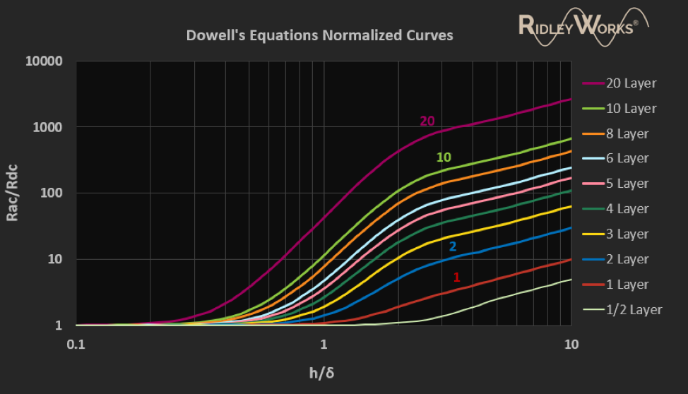
Figure 3: These curves completely represent the solution to Dowell’s equations for every design
Although the curves are an elegant and very compact representation of Dowell’s equation, it can be quite complex for newcomers to magnetics design to understand how to use them. The unexpected consequences of these curves cannot immediately be seen. We must apply the curves to specific situations to realize their full potential.
The first thing that you will notice about the curves is that the x axis does not plot frequency as a variable. Instead, it plots the height of the wire divided by the skin depth. Frequency is an implicitvariable, not explicit, since the skin depth given in Figure 1 is a function of frequency. Hence there is a double normalization in the x axis – the size of the wire chosen, and the skin depth at a given frequency. Observant engineers will also notice that the final slope of each of the curves is unity.
It is useful and instructional to take a more specific case and plot the curves as an explicit function of frequency. To do this, we have to select a layer height (in this case the thickness of a #29 wire) and center the curves around the frequency where h/δ is one. The example in figure 4 shows this to be 100 kHz. This is the frequency where the wire diameter is equal to one skin depth.

Figure 4: Plotting Dowell’s equation versus frequency
The range of frequencies that you can see in this form of the curves spans 4 decades, not just the two decades that you see with standard Dowell’s curves. 1 kHz to 10 MHz is a wide enough range to cover just about any need for modern power electronics. You can also see that the final slope is now 0.5, not unity as it is for the previous curves. Both of these effects are due to the fact that the skin depth is proportional to the reciprocal of the square root of the operating frequency.
If the wire gauge changes in your design, simply find the frequency at which one skin depth is equal to the new wire height. This becomes the central frequency of the set of curves. Notice that the underlying data of the curves does not change – only the x axis changes. There is no need to resolve the original equation. A fixed data set is sufficient.
Single Versus Multiple Layers
The curves for Dowell’s equation clearly show the penalty in using multiple layers of windings. They don’t reveal the whole story by inspection, however, since the y axis is normalized with respect to the dc resistance. When the winding layer count increases, the dc resistance will drop, and there is a vertical shift to the curve. This is best illustrated with a design example.
Consider the current waveform, and the two different winding designs in Figure 5.
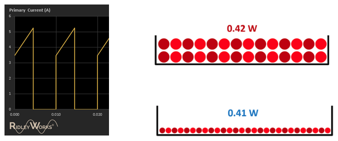
Figure 5: Primary current waveform and two different winding choices
In the upper winding arrangement of Figure 5, 2 layers of wire are used. Seven turns of 2x20 awg wire are used to make a 14-turn primary. In the lower winding arrangement, all of the turns are kept on a single layer. In order to fit the wire on the single layer, 2x26 awg wire are used. This means that the wire has only ¼ of the cross-sectional area of the two-layer winding.
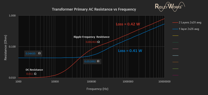
Figure 6: Un-normalizing the y axis for a specific design shows the power of Dowell’s analysis applied to different winding arrangements. In this example we have 4x less copper in the single layer winding, but the same dissipation.
As you can see in figure 6, the two-layer winding starts out with four times less resistance than the single-layer winding. However, at the switching frequency, the two-layer winding has a higherresistance. When we consider both the dc and ac components of the current flowing in the winding, the losses in these two different designs are just about the same. The one-layer design will be lower cost with lower capacitance. It provides a better engineering solution, although it conflicts with our natural intuition on design performance.
Foil Windings with Different Thicknesses
Even more dramatic effects can be seen if a winding is constructed of copper foil rather than wire. As the turns count drops, it becomes impractical to wind heavy gauge wire to fill the layer of a bobbin. Copper foil has been available to optimize this situation for over 100 years, and you will see this in old transformers with lower output voltages.
In Figure 7 you can see a foil winding on the left where the gauge of the copper has been chosen to completely fill the available bobbin area. The winding on the right has selected a thickness of foil to minimize the loss of the winding for the given waveform.
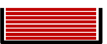
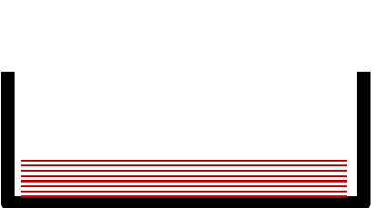
Figure 7: Two different foil windings. 50 mil foil is used on the left, and 6 mil foil is used on the right.
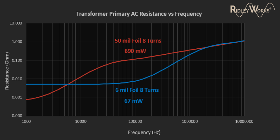
Figure 8: Dowell’s curves applied to the foil windings. The thin foil winding has over 15 times less dissipation than the winding, which is more than 8 times larger
As we can see from Figure 8, the thicker foil winding has about 8 times less resistance than the thin foil, as we would expect. However, at the switching frequency, the thick foil has almost 15 times moreresistance than the thin foil. The net result, when we take the currents at dc and the switching frequency and above, is more than a 10:1 reduction in loss with thin foil.
This is powerful knowledge to have when designing transformers and inductors. Once you realize that using less copper is often much more efficient, there are many opportunities for improving your magnetics design. For this foil case, we now have the option of increasing the spacing between the layers, resulting in a lower capacitance design. The thinner foil will also result in lower leakage inductance to other windings of the transformer.
Every winding design provides a different case to for analysis with Dowell’s curves. There is no standard solution. In every case, it is necessary to analyze the parameters and optimize the layers and gauges accordingly to minimize losses.
Summary
Published long ago, Dowell’s equations provided a powerful analytical tool for magnetics engineers. Without this type of analysis, dissipations in windings can be grossly in error. However, the equations are not widely used in the modern day since it is not reasonable to expect most working engineers to solve them. Today’s design schedules do not allow the time to properly understand and apply the theory. Fortunately, the numerical curves of Dowell’s equations contain all the results needed. Taking the time to learn how to read and apply the curves can make a tremendous difference to magnetics performance.
For interested engineers who want to speed up their learning and application further, the software used to generate the curves and waveforms in this article is available to the design community.[2]
References
[1] Magnetics Design Videos and Articles, Ridley Engineering Design Center.
[2] RidleyWorks™design software contains complete magnetics design and advanced analysis. A free Buck Designer is available to download.
[3] Learn about proximity losses and magnetics design in our hands-on workshops for power supply design www.ridleyengineering.com/workshops.html This is the only hands-on magnetics seminar in the world.
[4] Join over 4,000 engineers on our Facebook group titled Power Supply Design Center. Advanced in-depth discussion group for all topics related to power supply design.